As such, the three of them support mostly the same syntax (even if Scilab puts less emphasis on syntactic compatibility with MATLAB than Octave does).
From now on, the specific tool being used among the two MATLAB alternatives will not be specifically mentioned (mentioning "the tool" instead). We tried both alternatives and had more issues (build/installation, proper display) with Scilab, so we mostly used Octave, but did not find it very user-friendly.
Syntax
Putting a semicolon at the end of statement prevents the console from printing the corresponding value (answer, variable assignment, etc.).
Value Ranges
Ranges can be expressed thanks to:
- MIN:STEP_SIZE:MAX, like in: x = -10:2:10 resulting in 11 points
- or linspace(MIN, MAX, STEP_COUNT), like in: x = linspace(-10, 10, 11) to produce the same list as before
Array-based Functions
Many functions are defined so that they can be called also with arrays of parameters, instead of just standalone values. For that, a dot/period-based syntax has been introduced so that each element of an input vector is applied to the function in turn. A key understanding is that such a dot applies not to variables but to operators; for example 2*x.^2+1 shall not be read as 2*(x.)^2+1 but as 2*x(.^)2+1.
As an example, a \(\phi\) function can be defined as \(\phi(x) = e^{x}/(1+e^{x})\):
function retval = phi (x)
 retval = exp(x)./(1+exp(x));
endfunction
Then this function can be called either with a standalone value:
phi(1)
ans = 0.7311
or with an array thereof (a vector):
phi([1,2])
ans =
  0.7311   0.8808
Outputs
Beware to the lower-precision of textual outputs, which may be misleading (e.g. use format long with Octave to request 15 significant figures).
Script Files
Rather than being directly interpreted (e.g. from a pasted text), a series of statements can be gathered in a script file (a bit different from a function file ) that can be loaded and executed afterwards.
Their conventional extension in m (e.g. foobar.m), due to the MATLAB legacy.
Avoid dashes in the script filenames, as it may be interpreted as minus; prefer underscores (e.g. phi_exp.m rather than phi-exp.m).
An example of script, named phi_exp.m:
# An initial comment prevents Octave from thinking that this
# is a function file:
1;

# The function name can be freely chosen, it does not have to
# correspond to the script filename:
#
function retval = phi_exp (x)
   retval = exp(x) ./ (1+exp(x))
endfunction

xs = -10:10
ys = phi_exp(xs)

plot(xs,ys)

title ("A function phi to map values V to a probability-suitable ]0,1[ interval")
ylabel ("\phi(V)")
xlabel ("V")
grid on
Provided that such a script is located in a well-known directory of the tool (typically its working directory), it can be executed simply by entering its filename without extension; for example:
octave:1> phi_exp
warning: function 'phi_exp' defined within script file 'xxx/phi_exp.m'
xs =
 -10   -9   -8   [...]
Then a script can be run from the command-line; for example:
$ octave --eval phi_exp.m --persist
# OR
$ octave phi_exp.m
Scilab may be best obtained, on Arch Linux, from the AUR (e.g. yay -Sy scilab) by selecting the scilab-bin option (relying then on prebuilt binaries); it can then be run with: scilab.
We experienced quite a few issues in order to obtain Scilab by any means. A last-resort option is to rely on an AppImage instead; one may then sandbox it: first the Scilab AppImage shall be downloaded, for example as ~/Scilab-x86_64.AppImage. Then:
$ mkdir -p ~/Software/scilab
$ cd ~/Software/scilab
$ mv ~/Scilab-x86_64.AppImage .
$ chmod +x Scilab-x86_64.AppImage
$ firejail --appimage ./Scilab-x86_64.AppImage &
Once installed that way, our run-scilab.sh can be used instead.
Note that the copy/paste behaviour is not consistent with the usual UNIX/X11 one, and that tabulation can be used for auto-completion.
Scilab does not seem to offer any symbolic support out of the box. See Using Maxima instead (knowing that Maxima may be integrated within Scilab).
Defining a Function
Let's suppose we want to define \(my\_func: x \rightarrow 2.x^{2}+1\).
For that, in Scilab's shell, enter:
--> function [y] = my_func(x)
  > y = 2*x^2+1
  > endfunction
Then:
--> my_func(5)
 ans  =
   51.
Plotting a Function
Let's define the support of our function, here computed from 0 to 10 with 50 values: my_xs = linspace(0, 10, 50). Then just execute plot(my_xs, my_func).
We experienced rendering issues that prevented a proper display of plots.
Octave can be installed on Arch Linux with pacman -Sy octave; extra packages may be needed (e.g. octave-quaternion, available in the AUR).
The command-line version can be run as octave. Typing quit at the prompt allows to exit.
The GUI version can be launched with octave --force-gui.
Defining a Function
As already seen, so that it can operate on single values or arrays, a \(\phi(x) = e^{x}/(1+e^{x})\) function can be defined as:
function retval = phi (x)
  retval = exp(x)./(1+exp(x))
endfunction
Plotting a Function
We consider first a function of a single variable.
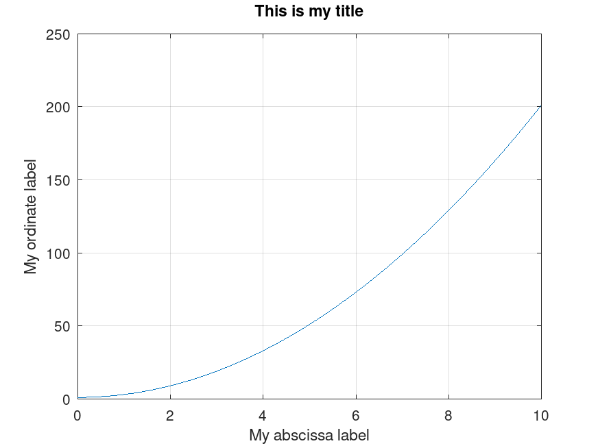
Let my_xs = 0:0.2:10 define the support / display range of our function; then:
my_ys = my_func(my_xs)
plot(my_xs, my_ys)
A key point is to understand that, for all plots (plot, mesh, surf, etc.), the last element to be specified is not the function to which the previous elements are to be applied, but directly the final values to plot.
Extra display settings can be added afterwards:
title ("This is my title")
ylabel ("My ordinate label")
xlabel ("My abscissa label")
grid on
This results in:

The image can be saved either by using the Save As GUI menu and typically selecting PNG, or directly from the console/scripts thanks to the following command: print("my_plot.png", "-dpng").
Maxima is a free software (GPL) tool for the manipulation of symbolic and numerical expressions.
It can be installed on Arch with pacman -Sy maxima.
A graphical frontend exists, considerably more user-friendly, and useful for teaching the use of Maxima: wxmaxima; it is available on the Arch AUR, yet its build fails at the time of this writing; it has however an AppImage - just try to find a recent wxmaxima-x86_64.AppImage there.
One may then store this image in ~/Software/maxima/ and run it either directly or in a sandboxed environment: firejail --appimage wxmaxima-x86_64.AppImage; see also our run-maxima.sh script.
For example, taking into account that (refer to this introduction for more details):
- to assign a value to a variable, use the colon (: ; for example: a : [1,2]), not the equal sign (that is used for representing equations)
- each statement is to be ended, on:
- the command-line: with a semi-colon (;) followed by Enter
- the GUI: with just Shift-Enter (the semi-colon is auto-added; Enter is used here for multiline inputs)
- one shall enter quit(); to exit
- a general matrix m may be defined that way:
m: matrix(
 [m11,m12,m13,tx],
 [m21,m22,m23,ty],
 [m31,m32,m33,tz],
 [0,0,0,1]
);
- a diagonal matrix s may be defined that way:
s: matrix(
 [Sx,0,0,0],
 [0,Sy,0,0],
 [0,0,Sz,0],
 [0,0,0,1]
);
- a diagonal matrix t may be defined that way:
t: matrix(
 [1,0,0,trx],
 [0,1,0,try],
 [0,0,1,trz],
 [0,0,0,1]
);
- multiplication is represented by a dot : m.s;
then Maxima can be directly used in a terminal:
$ maxima
;;; Loading #P"/usr/lib/ecl-23.9.9/sb-bsd-sockets.fas"
;;; Loading #P"/usr/lib/ecl-23.9.9/sockets.fas"
Maxima 5.47.0 https://maxima.sourceforge.io
using Lisp ECL 23.9.9
Distributed under the GNU Public License. See the file COPYING.
Dedicated to the memory of William Schelter.
The function bug_report() provides bug reporting information.
[...]
(%i1) m: matrix(
 [m11,m12,m13,tx],
 [m21,m22,m23,ty],
 [m31,m32,m33,tz],
 [0,0,0,1]
);
                            [ m11  m12  m13  tx ]
                            [                   ]
                            [ m21  m22  m23  ty ]
(%o1)                       [                   ]
                            [ m31  m32  m33  tz ]
                            [                   ]
                            [  0    0    0   1  ]
(%i2) s: matrix(
 [Sx,0,0,0],
 [0,Sy,0,0],
 [0,0,Sz,0],
 [0,0,0,1]
);
                              [ Sx  0   0   0 ]
                              [               ]
                              [ 0   Sy  0   0 ]
(%o2)                         [               ]
                              [ 0   0   Sz  0 ]
                              [               ]
                              [ 0   0   0   1 ]
(%i3) m.s;
                       [ Sx m11  Sy m12  Sz m13  tx ]
                       [                            ]
                       [ Sx m21  Sy m22  Sz m23  ty ]
(%o3)                  [                            ]
                       [ Sx m31  Sy m32  Sz m33  tz ]
                       [                            ]
                       [   0       0       0     1  ]
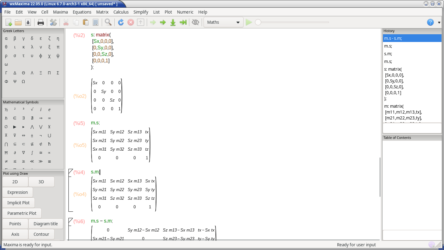
Doing the same this time with wxmaxima:

A session can be saved in a file, using the *.wxmx extension.
See also Maxima's documentation.

